Nearest Neighbor Search Algorithms: An Intro to KNN and ANN

Nearest Neighbor Search Algorithms

Rapid advancements in AI have made machine learning mainstream, introducing developers everywhere to a whirlwind of new tools, techniques, and terminology. This blog explores nearest neighbor algorithms - specifically, the exact k-Nearest Neighbor (KNN) search algorithm, as well as the Approximate Nearest Neighbor (ANN) search, a variant of kNN that trades accuracy for speed.

Why Vector Search?

From early cancer detection to your “Discover Weekly” Spotify playlists, today’s cutting-edge technologies and personalized experiences rely on vector searches. Lucky for us, many databases now either support vector storage and search, or are specifically designed for that purpose.

Whether you're using a database with native vector support (like Rockset, Elasticsearch, or Pinecone) or one that offers it through extensions (such as Postgres with pg_vector), grasping the core algorithms behind a vector search is essential for creating robust AI applications.

In today’s blog, we’ll unpack how vector searches work. We’ll examine the traditional exact k-Nearest Neighbor algorithm, as well as an optimized variant that trades precision for performance. You will surely leave today with enough know-how to start building AI applications on top of your vector store of choice. Without further ado, let’s get started!

A Brief Intro to Vectors and Vector Search

If you’re new to the concept of vectors or vector search, we recommend checking out this article on the topic. In short, a vector is a sequence of numbers that represent a point in a multi-dimensional space. Advanced machine learning architectures, such as BERT for text data, transform unstructured inputs into vector representations termed "embeddings". These embeddings encapsulate semantic nuances decipherable by computational algorithms, and their spatial orientations with respect to other embeddings signifies inherent associations or relationships. The closer two points are, the more similar they are. We can leverage these associations to perform classifications, regressions, and other ML tasks.

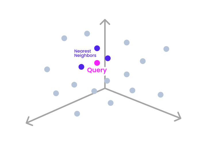
If we examine the space around a new embedding (a query point), we can find its nearest “neighbors”. The traditional exact k-NN algorithm identifies the k exact nearest embeddings to the query point. Approximate Nearest Neighbor algorithms also find k neighbors, but they relax the precision requirement, which allows for performance optimizations.

We’ll focus on the exact k-NN algorithm first, before moving onto modern approaches like ANN.

The Exact K-Nearest Neighbors Algorithm

k-Nearest Neighbors is a simple algorithm that finds the k exact nearest neighbors of a given query point (observation). k-NN is most often used to categorize observations based on nearby observations (classification), but it can also be used to predict a value associated with a new observation (regression). For example, we might want to determine if a piece of text is positive, negative, or neutral (a classification task known as sentiment analysis), or predict the value of a home given its attributes (a regression task).

Using the k-NN algorithm can be broken into these steps:

1. Choosing k 
2. Choosing a distance measurement
3. The actual query run on your vector dataset
4. The decision made to accomplish your specific task, based on the results of your query

Let’s take a closer look at each step.

Components of a k-NN

Choosing k

The first step of the k-NN algorithm is to choose k, or the number of neighbors you want to take into account when making a decision. Your choice of k is important. Too small, and your results may be noisy and sensitive to outliers. Too large, and it might pick up neighbors that are no longer representative of what you’re looking for. Cross-validation is a useful method to determine an optimal k.

Distance Measurements

Determining which k observations are returned depends on how you choose to measure distance between embeddings. The most common metric is Euclidean distance - a straight line in vector space between embeddings. Due to the linear nature of Euclidean distance, it’s important for your features to either be of a similar scale, or be normalized through feature scaling.

Euclidean distance is not preferred when working with high-dimensional data, as is the case with text data represented as vectors. This stems from the “curse of dimensionality”, a term which describes the challenges that emerge when dealing with high-dimensional spaces. One challenge, for example, is that as the number of dimensions grows, the volume of the vector space increases. As the vector space volume grows, vector spaces grow sparse. It’s a similar mental model to how the universe expands - as the volume of the universe grows, solar systems grow further apart and space gets less “dense”. As the vector space grows sparse, Euclidean distances between data points tend to converge, making it harder to distinguish between points and rendering this distance metric less effective for discerning similarities or differences.

Instead, you should consider cosine similarity, which measures how similar two vectors are based on the cosine angle between them. Because cosine similarity measures angle and not distance, cosine similarity can be an excellent choice for datasets with non-normalized features, or when dealing with high-dimensional vector data.

The Search

A brute-force approach to find k-nearest neighbors would calculate the distance of the new observation to every other observation. With O(n) time complexity, this is an expensive operation that could take a prohibitively long time on large datasets. Most vector stores implement a few optimizations to improve their k-NN search performance.

Spatial data structures are one common technique to improve on a brute-force k-NN. For low to moderate-dimensional data (typically less than 20 dimensions), kD trees can significantly speed up a vector search by partitioning the embeddings into hyperrectangles. Data is partitioned by the space it exists in, enabling searches to quickly eliminate large chunks of the dataset that are too far to be considered neighbors.

When choosing a database for your vector data, be sure to look into what optimization techniques are used to deliver high-performance queries.

Making a Decision

After k neighbors are retrieved, it’s time to perform a task. An exact k-NN search can be used to perform both classification and regression tasks, but there are typically better options to perform regression tasks, so we’ll look closer at classification.

The most common technique to classify a new observation is a simple majority vote mechanism among the k-nearest neighbors. So, in our sentiment analysis example, with a k of 5, if 3 of the 5 observations are labeled as positive, the new observation will be classified as positive.

There are a wide variety of use cases for a traditional exact k-NN search. If your dataset is large enough, however, you may need to consider alternatives to the traditional approach.

Approximate Nearest Neighbors

As a vector database grows to billions of vectors, or thousands of dimensions, calculating exact values starts to make less sense. On the one hand, as the number of vectors increases, the computational complexity skyrockets, making exact distance computations impractical and inefficient.

In cases where exactness isn’t necessary, and a good enough match will suffice, we can use Approximate Nearest Neighbor search, a performance-optimized approach to a k-NN search. While traditional k-NN might need to examine an entire dataset to guarantee finding the exact nearest neighbor, ANN algorithms can bypass certain sections of the search space or terminate early once a satisfactory match is identified. This leads to faster searches and lower computational requirements.

There are a variety of techniques to “narrow the focus” of a given similarity search. Some of these include locality-sensitive hashing (LSH), Hierarchical Navigable Small Worlds (HNSW), and product quantization. In general, when building your own ANN applications, you should reach for libraries like Facebook AI Similarity Search (FAISS) or Approximate Nearest Neighbors Oh Yeah (ANNOY). These libraries offer efficient similarity searches and clustering of dense vectors through algorithm- and hardware-based optimizations. They are designed to make use of GPU-based indexes, and provide mechanisms to read and write indexes to disk efficiently.

Use Cases and Guidelines for Nearest Neighbor Algorithms

Keep these in mind when evaluating nearest neighbor algorithms:

1. Accuracy vs Speed Tradeoff: Evaluate your latency requirements and your use cases tolerance for imprecise results. Find the right balance between speed and accuracy.
2. Dimensionality and Dataset size: Choosing the right algorithm often comes down to the number of dimensions you are working with, as well as the dataset size.
3. Quality of Embeddings and Representations: Irrelevant or redundant features can hamper the effectiveness of any k-NN search. Certain algorithmic optimizations are particularly vulnerable to poorly-curated features. Take the time to select the best features for your use case, and to normalize your data - this can significantly improve the quality of your ANN searches.

In general, if you are working with a few hundred thousand vectors with less than 50 dimensions, an exact k-NN approach will likely suffice. Use cases could include credit approvals, sentiment analysis, or medical diagnosis.

If your dataset is in the millions or billions of vector embeddings, with hundreds or thousands of dimensions, then a combination of feature engineering (normalization, scaling, etc to ensure high-quality features), dimensionality-reduction (to reduce the number of dimensions while maintaining similarity between vectors), and ANN libraries like FAISS and ANNOY are your best options. This covers use cases like large-scale searches of images, audio and text, real-time content feed generation, recommendation engines, anomaly detection and more.

Next Steps

It seems like new tools are being launched every day to simplify the process of creating AI-driven applications. In a coming blog post, we’ll use a single dataset to demonstrate three different kinds of tasks using k-NN, so make sure to subscribe for more content. In the meantime, tinkering is a great way to get started, and the below are some resources to help kick-start your journey with ML and k-NN searches.

If you want to get started building an application on top of a vector datastore, Rockset makes it simple to connect to a data source or upload your data and perform sub-millisecond queries on your vector data. Plus, features like query lambdas let you rapidly deploy APIs to consume and search your vector data. Learn more about Rockset as a vector database here.